Marching Cube Algorithm For Implicit Surface Plotting
Background
Equations in the form of are called implicit surface, e.g. is an implicit equation of the ellipsoid. Such equations are often arises in engineering and mathematics. It is helpful to visualize these equations to understand the system clearly or to communicate the idea with others. If we can convert an implicit equation to a parameteric equation the surface plotting task become easy, and computationally less expensive. However such transformation are not always possible. Therefore we need an algorithm that accept an arbitrary equation of implicit surface and bounding space as parameters, and generate surface within the bound. Ray tracing method is often used for this task. The other approach which we discuss here is to use marching cube. Though it suffers from some limitations, it has capability to plot arbitrary surface with acceptable deviation.
Marching Cube Algorithm
The algorithm divide the space in a finite number of small cube and evaluate the equation at the corner of each cube. The evaluated value can be either non-negative or negative (ignoring discontinuity), therefore there are possibilities. However half of them are reflection of the other half. Moreover if we notice carefully we see there are only fifteen different combinations that we need to care about. They are shown in the following figure.
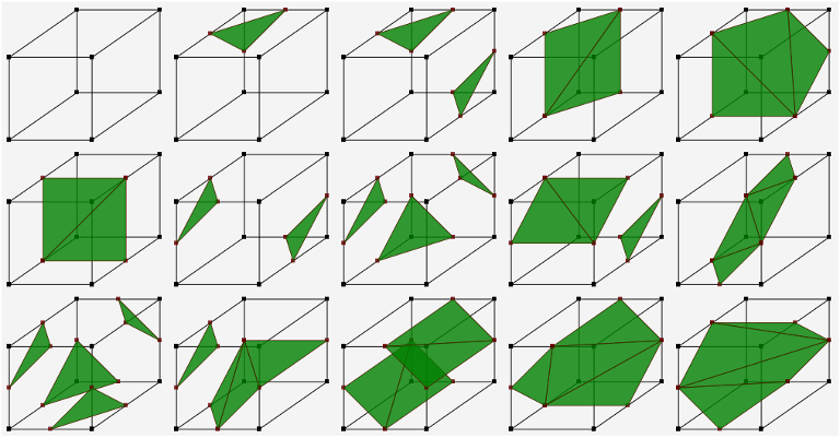 Figure 1: Fifteen possible unique combination of vertices
Similar to marching square we have to some ambiguous configuration too - first and third configuration in the last. Here we also have to take care of the topology of the surface, that is our algorithm should not produce holes in the surface. Moreover, if we want to add lighting support for the surface so that it looks nice instead of patches of triangles we have to add surface normals at each vertex. Finally we can extend idea of quadtree to create a more robust octet tree surface plotting algorithm. However unlike quadtree where number of leaf node grows exponentially by a factor of 4, the condition is even worse, the tree will grow exponentially by a factor of 8. That is at the depth of six we have nodes and about function evaluations - no visual rendering at all!
Handling configurations efficiently
To handle the configuration efficiently we use bit-wise trick, we pack the sign information of vertices in a 8-bit integer. By doing so we get a number between 0 and 255(both inclusive). We assign a number between 0 and 7 to each vertex and between 0 and 11 to each edge. We create a lookup table which gives information about the edges that are the part of the triangular patches for each of 256 configurations. In particular the look up table will store a list of edges in the multiple of three. These edges tell that which two vertices we need to interpolate. The total size of table is bounded above by , as each entry in the table may have at most 12 edges, that is space complexity is still small as compared to time complexity of the algorithm. Though we can’t visualize in higher dimension but complexity of space partitioning based algorithms increases exponentially as more and more dimension is added.
I haven’t included the code to avoid mess, however I have already uploaded configuration table to github.If you need full code you can browse Geogebra Library. Maybe soon I would upload some javascript based demo using threee.js framework as WebGL engine.
Results
The implemented algorithm can plot a wide range of equation. However it fails to plot surface with singularities and sometimes ends up with missing a whole patch of the surface. I have included some outputs of the algorithm [see fig]. The second plot looks quite like an ellipsoid and in fact it is! When we take log both side of the equation and manipulate it a little bit we get an equation of ellipsiod. Similarly contour of gaussing with two variable in is an ellipse.
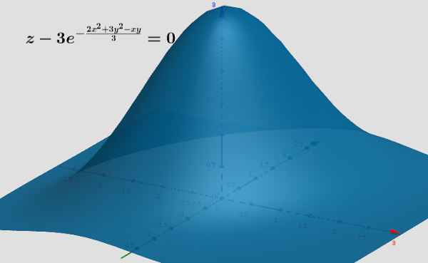 Figure 1: Implicit surface of gaussian with two variable (not-normalized)
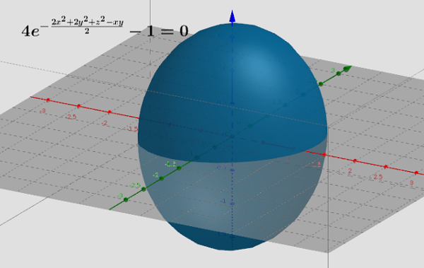 Figure 1: You can interprete it as a contour surface of gaussian with three variables