Intersection between Implicit Curves

Interscetion between two implicit curves

I worked with GeoGebra during summer 2015, and implemented some functionality including intersection of implicit curves. The experience were exciting, and I learnt significantly. Here I would like to share a some of them, hope it may help you. Anyway finding intersection between simple curves are far easy; however, when we have to implement functionality that work well with a wide range of implicit equations the task becomes partially intractable and needs sophisticated approach to deal with edge and corner cases. Particularly, in this post I would discuss two different method to find intersection between two implicit curves $f(x, y) = 0$ and $g(x, y) = 0$ . I would start with simple problem formulation, manual solution followed by two methods - Newton’s and Broyden’s method to find intersections.

Problem formulation

For two different implicit curves $f(x, y) = 0$ and $g(x, y) = 0$ find some points $(x_k, y_k)$ , where $x_{min} \le x_k \le x_{max}$ and $y_{min} \le y_k \le y_{max}$ , in $\mathbb{R}^2$ such that $f(x_k, y_k) = 0$ and $g(x_k, y_k) = 0$ .

Example

Let $f(x, y) = y - x^2 - 4 = 0$ and $g(x, y) = y - 2x^2 = 0$ . From second equation we get $y = 2x^2$ . When we substitute this value in the first equation we get $x = \pm 2$ . Thus $(x, y) = \{(-2, 8), (2, 8)\}$ satisfies both equation. But, it is not always so simple. It is difficult to find the solution of $x^3 + 3x^2y + 5xy^2 + 4xy + y^3 = 0$ and $sin(x + 2y) + xy = 0$ .

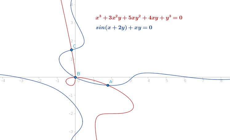
Figure 1: Intersection example (in GeoGebra Beta): This was a fun and relatively hard example with any root near zero converges slowly towards zero. Also notice that the red curve has a singular point at origin and there exists root at origin but the jacobian matrix at origin is singular which makes the problem difficult.

Newton’s Method

Newton’s method is an iterative method which is used to find roots of function $f(x) = 0$ . In this method we begin with some intial guess $x_0$ and iteratively update initial guess with a better approximation using following expression until desired accuracy is achieved

$x_{k+1} = x_{k} - \frac {f(x_k)} {f'(x_k)}$

The same idea can be extended to $\mathbb{R}^2$ find intersection between two implicit curves. we know that

$f(x + \Delta x, y + \Delta y) = f(x, y) + [\frac {\partial f(x, y)} {\partial x}, \frac {\partial f(x, y)} {\partial y}] [\Delta x, \Delta y]^T + O(\epsilon^2)$

We begin with some intial guess $(x, y)$ , and try to move small step $(\Delta x, \Delta y)$ in the best direction that is the move for which $f(x + \Delta x, y + \Delta y) \approx g(x + \Delta x, y + \Delta y) \approx 0$ .

To avoid clutter let’s define

$\Delta x = x_{k+1} - x_k$ , $\Delta y = y_{k+1} - y_k$ , $f(x, y) = f_k$ , $f(x + \Delta x, y + \Delta y) = f_{k+1}$ , $\partial f(x, y) /\partial x = f_x$ , $\partial f(x, y) /\partial y = f_y$ , and the same for g(x). We can write

$F = - J \Delta X$ $\Rightarrow \Delta X = -J^{-1} F$

where $F = \begin{bmatrix}f_k & g_k\end{bmatrix}^T, \Delta X = \begin{bmatrix}\Delta x & \Delta y \end{bmatrix}^T$ , and

$J = \begin{bmatrix} f_x & f_y \\ g_x & g_y \end{bmatrix}$

Since $J$ is a 2x2 square matrix it is simple to find its inverse.

$J^{-1} = \frac{1} {f_xg_y - g_xf_y} \begin{bmatrix} g_y & -f_y \\ -g_x & f_x \end{bmatrix}$

Now the expression becomes

$\begin{bmatrix} x_{k+1} \\ y_{k+1} \end{bmatrix} = \begin{bmatrix} x_{k} \\ y_{k} \end{bmatrix} - \frac{1} {f_xg_y - g_xf_y} \begin{bmatrix} g_y & -f_y \\ -g_x & f_x \end{bmatrix} \begin{bmatrix} f_{k} \\ g_{k} \end{bmatrix}$

Where ${f_xg_y - g_xf_y} \ne 0$

The idea can be extended to equation even in higher dimension.

Browse code here

 
// java code for the intersection of implicit curves
public class Solver {

    public static interface FunctionXY {
        public double evaluate(double x, double y);
        public double derivativeX(double x, double y);
        public double derivativeY(double x, double y);
    }

    public static boolean isZero(double v, double eps) {
        return (v > -eps) && (v < eps);
    }

    public static void add(List<double[]> sols, double x, double y) {
        for(int i = 0; i < sols.size(); i++) {
            double[] v = sols.get(i);
            if(isZero(x - v[0], 1e-6) && isZero(y - v[1], 1e-6)) {
                return;
            }
        }
        sols.add(new double[]{x, y});
    }

    public static List<double[]> solve(FunctionXY f, FunctionXY g, 
        double[] bounds, double eps) {
        double[][] samples = rootSamples(f, g, bounds, 10, 10);
        List<double[]> sols = new ArrayList<>();
        double x1, y1, x2, y2, er, er1, fv, gv, fv1, gv1;
        double jfx, jfy, jgx, jgy, det, alpha, dx, dy;
        int MAX_ITR = 8;
        boolean success;
        for(int i = 0; i < samples.length; i++) {
            x1 = samples[i][0];
            y1 = samples[i][1];
            fv = f.evaluate(x1, y1);
            gv = g.evaluate(x1, y1);
            er = Math.abs(fv) + Math.abs(gv);
            for(int j = 0; j < MAX_ITR && !isZero(er, eps); j++) {
                jfx = f.derivativeX(x1, y1);
                jfy = f.derivativeY(x1, y1);
                jgx = g.derivativeX(x1, y1);
                jgy = g.derivativeY(x1, y1);
                det = jfx * jgy - jfy * jgx;
                if(isZero(det, 1e-8)) {
                    break;
                }
                dx = (jgy * fv - jfy * gv) / det;
                dy = (jfx * fv - jgx * gv) / det;
                alpha = 1.0;
                success = false;
                // We can use line search that satisfies
                // Wolfe condition, but for now keep it
                // simple
                do {
                    x2 = x1 - dx;
                    y2 = y1 - dy;
                    fv1 = f.evaluate(x2, y2);
                    gv1 = f.evaluate(x2, y2);
                    er1 = Math.abs(fv1) + Math.abs(gv1);
                    if(er1 < er) {
                        success = true;
                        // variable exchange
                        break;
                    }
                    alpha *= 0.8;
                } while(alpha >= 0.01);

                if(!success) break;
            }

            if(isZero(er, eps)) {
                add(sols, x1, y1);
            }
        }
        return sols;
    }

    /**
     * divide the entire space in 10x10 grid and evaluate
     * f and g at each vertex return mid point of consecutive
     * vertices for which both functions change their sign.
     */
    public double[][] rootSamples(FunctionXY f, FunctionXY g, double[] bounds,
            int sampleXSize, int sampleYSize) {
        return null;
    }
}

Damping

You maight have noticed that in each iteration algorithm starts with full step size and reduces it until the error become smaller than the previous error or the move becomes too small. It is necessary because sometimes the step size $\Delta X$ that is chosen by the algorithm is too large that leads to divergence. To avoid it we introduce a damping factor $\alpha$

$X_{k+1} = X_{k} - \alpha J^{-1} F_k,$ where $0 \lt \alpha \le 1$

Do $\alpha > 1$ be a good choice of damping factor? Let’s take an example of $f(x, y) = y - x^2 = 0$ and $g(x, y) = x - y^2 = 0$ . When we start from point $(-1, -1)$ the step size without damping is $(2/3, 2/3)$ . If we take $\alpha = 1.5$ or $\alpha = 3.0$ we reach at the root in a single step. Therefore which is a good value : $0 \lt \alpha \le 1$ , $\alpha = 1.5$ or $\alpha = 3.0$ . In our example seemingly $\alpha \gt 1.0$ is a better choice than $\alpha \le 1$ . However look at the figure-2, when we start at point $A$ the full step length leads to point $C$ far from the solution, at $\alpha \approx 0.4$ (chosen heuristically) we get point $B$ which is close to the solution. For an arbitray unknown equation there is no known good way to select the exact value of $\alpha$ . We assume that the function is continuous in the neiborhood, and try to move in the direction that may have solution. A long jump may violet our initial assumption. Furhtermore when we bound the range of $\alpha$ we can apply search heuristic to find better value.

Read here about damping related tricks and optimization

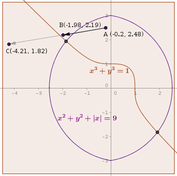
Figure 2: Line search for good value of $\alpha$

Selecting Damping Factor

There are several approaches to select damping factor $\alpha$ we can use quadratic interpolation, line search, binary search, quadratic decay rate, (will post more about it soon)

Convergence of Newton’s Method

Let’s begin with an intuitive discussion. Suppose both functions, $f(x, y)$ and $g(x, y)$ are linear bivariate function. That is, $f(x, y) = a_1x+b_1y+c_1=0$ and $g(x, y) = a_2x+b_2y+c_2 = 0$ . Since the higher order error term $O(\epsilon^2)$ is zero, Newton’s method should produce the correct answer in a single iteration as long as jacobian matrix $\mathbf{J}$ is invertible. Following derivation shows that in fact it does give the solution in a single step. Notice that the end result is nothing but the solution that we get by directly applying Cramer’s rule.

$\mathbf{J} = \begin{bmatrix} a_1 & b_1 \\ a_2 & b_2 \end{bmatrix}$

If the inital guess is $(x_k, y_k)$ then

$\begin{bmatrix} x_{k+1} \\ y_{k+1} \end{bmatrix} =$ $\begin{bmatrix} x_k \\ y_k \end{bmatrix} - {\begin{bmatrix} a_1 & b_1 \\ a_2 & b_2 \end{bmatrix}}^{-1} \begin{bmatrix} f_k \\ g_k \end{bmatrix} =$ $\begin{bmatrix} x_k \\ y_k \end{bmatrix} - \frac {1} {a_1b_2 - a_2b_1}$ $\begin{bmatrix} b_2 & -b_1 \\ -a_2 & a_1 \end{bmatrix}$ $\begin{bmatrix} a_1x_k + b_1y_k + c_1 \\ a_2x_k + b_2y_k + c_2 \end{bmatrix}$

$\Rightarrow \begin{bmatrix} x_{k+1} \\ y_{k+1} \end {bmatrix} =$ $\frac {1} {a_1b_2 - a_2b_1} \begin{bmatrix} c_2b_1 - c_1b_2 \\ a_2c_1 - a_1c_2 \end{bmatrix}$

We have seen that in case of linear implicit equation Newton’s method converges in one iteration. In general case the behaviour depends upon the error term $O(\epsilon^2)$ . That is one of the reasons we use damping factor $\alpha$ - we never want divergence of error. So when we choose the gradient direction $\mathbf{p}$ to move in, we also ensure that the error doesn’t exceed the previous error. If it does we reduce (damp) the direction by $\alpha$ . You might be thinking about how we can choose a good direction, how much we should damp, and how we can ensure that damping would not help to reach at solution. As in following equation

$f(x, y) = x^2 - 2xy + y^2 + 10^{-6} = 0$ $g(x, y) = -x^2 + 2xy - y^2 - 10^{-6} = 0$

You may try to visualize the graph. (Edit: No real value of $x$ and $y$ satisfies any of the above equation, though at $(x, y) = (0, 0)$ the left side is very close to zero.)

Limitations

For implicit curve both functions should be smooth in $\mathbb{R}^2$ and differentiable
It is computationally expensive to evaluate derivative at each step
Near singular jacobian matrix sometimes leads to divergence
If starting point is not close to the solution, the algorithm may not converge quickly or even may diverge

Broyden’s Method

Broyden’s method, originally described by CG Broyden, is a quasi-Newton method for root finding. In contrast to Newton’s method, in which we have to calculate jacobian matrix $\mathbf{J}$ in each iteration, we calculate jacobian only in the first iteration and we do rank one update in other iterations. Broyden’s method converges to solution in $2n$ iterations for linear system, however it may even fail to converge for non-linear system of equation.

We start with the idea of secant method for one variable. The finite difference approximation of $f(x)$ is given by

$f'(x_n) = \frac {f(x_n) - f(x_{n-1})} {x_n - x_{n-1}} = \frac {\Delta f(x_n)} {\Delta x_n}$

When we substitute this value to Newton iteration, we get

$x_{n+1} = x_n - \frac {f(x_n)} {f'(x_n)}$

To develop intuition about how we can update $f'(x_n)$ from $f'(x_{n-1})$ let’s start with following expression all in $\mathbb {R}$

$f'(x_n) = \frac {\Delta f(x_n)} {\Delta x_n} = f'(x_{n-1}) + \frac {\Delta f(x_n) - f'(x_{n-1}) \Delta x_n} {\Delta x_n}$

Here it seems absurd to expand middle term to get right hand side expression. But we notice that in the middle term we are directly calculating $f'(x_n)$ but in right hand side we are updating previous derivative to get new one.

A failed attempt

To extend the idea let us define following notations in $\mathbb {R}^n$

$\mathbf {x} = (x_1, x_2, \dots, x_n)$ $\mathbf {f} = (f_1(x_1, x_2, \dots, x_n), f_2(x_1, x_2, \dots, x_n), \dots, f_n(x_1, x_2, \dots, x_n))$

The secant equation using jacobian matrix can be written as

$\mathbf {J_n(x_n-x_{n-1})=f(x_n) - f(x_{n-1})}$

To reduce clutters we define $\mathbf {f_n = f(x_n)}$ , $\mathbf {\Delta x_n = x_n-x_{n-1}}$ and $\mathbf {\Delta f_n = f(x_n) - f(x_{n-1})}$

Now using new notations we can write

$\mathbf {J_n\Delta x_n = \Delta f_n}$ $\Rightarrow \mathbf {J_n = \Delta f_n \Delta {x_n}^T (\Delta x_n \Delta {x_n}^T)^{-1}}$

We can see that,

$\mathbf {\Delta f_n \Delta x^T = J_{n-1} \Delta x \Delta x^T + \Delta f_n \Delta x^T - J_{n-1} \Delta x \Delta x^T}$ $\Rightarrow \mathbf {\Delta f_n \Delta {x_n}^T = (J_{n-1} + \frac {\Delta f_n - J_{n-1} \Delta x_n} {\Delta {x_n}^T \Delta x_n} \Delta {x_n}^T) (\Delta x_n \Delta {x_n}^T) }$

Therefore,

$\mathbf {J_n = \Delta f_n \Delta {x_n}^T (\Delta x_n \Delta {x_n}^T)^{-1} = J_{n-1} + \frac {\Delta f_n - J_{n-1} \Delta x_n} {\Delta {x_n}^T \Delta x_n} \Delta {x_n}^T}$

Alternatively we can use Sherman-Morrison formula to find directly inverse of Jacobian matrix:

$\mathbf {H_n = H_{n-1}+ \frac {\Delta x_n - H_{n-1} \Delta f_n} {\Delta {x_n}^T H_{n-1} \Delta f_n} \Delta {x_n}^T \Delta H_{n-1}}$

where $\mathbf {H_n = J_n^{-1}}$

Though the final expression for the rank-one jacobian update is a valid expression the steps that lead to it is not valid. Notice the $\mathbf {\Delta x_n \Delta {x_n}^T}$ is a singular matrix therefore it is not invertible. Suppose for a moment that it is invertible, to reach at conclusion we have added and substracted previous jacobian $\mathbf {J_{n-1}}$ . Why do we have chosen the previous jacobian? We may have selected a null matrix or nothing at all. What the last expression is actually doing?

Let’s start from scratch, in Newton’s Method the next good approximation is given by following expression

$\mathbf {x_{i+1} = x_i - J^{-1}\Delta f_i}$

and to prevent divergence we use $\mathbf {x = x_i + t\Delta x_i}$ , where $t$ can take any value. Now each function can be regarded as a function of single variable namely $t$ and we would like to find an optimum value of it. Since partial derivative is assumed to exist we can take partial derivative of each function with respect to $t$ and applying chain rule we can write -

$\frac {\partial {f_i}} {\partial{t}} = \sum_{k=1}^{n} \frac{\partial f_i} {\partial x_k} \frac {dx_k}{dt}$ $\Rightarrow \mathbf {\frac{df}{dt} = J\Delta x_i}$

Hence if an accurate estimate of $\mathbf {\frac{df}{dt}}$ availabe we can approximate jacobian matrix $\mathbf {J}$ . For now assuming $\mathbf {f}$ only function of $t$ Taylor series expansion about $t$ ignoring higher order terms can be written as

$\mathbf {f(t - s) \approx f_{i+1} - s\frac{df}{dt}}$ $\Rightarrow \mathbf{f_{i+1} - f(t_i-s_i) = s_iJ\Delta x_i}$

The last equation relates to four already known quantities to fifth $\mathbf {J}$ to which an approximation $\mathbf{B_i}$ is available and to which a new estimation $\mathbf {B_{i+1}}$ is sought. In the class of method explained by Broyden $\mathbf{B_{i+1}}$ is chosen in such a way as to satisfy the equation

$\mathbf {f_{i+1} - f(t_i-s_i) = s_iB_{i+1}\Delta {x_i}}$

The above expression relates the change in function vector to change of $\mathbf {x}$ in the direction of $\mathbf {\Delta x}$ , there is no information available about the behavior of function in other directions. Therefore it is not possible to obtain fresh rate of change in these directions. According to the first method suggested by Broyden $\mathbf{B_{i+1}}$ chosen so that the change is $\mathbf{f}$ predicted by $\mathbf {B_{i+1}}$ in a direction $\mathbf {q_i}$ orthogonal to $\mathbf {\Delta x_i}$ is the same as would be predicted by $\mathbf{B_i}$ . Symbolically,

$\mathbf {B_{i+1}q_i = B_iq_i}$ $\mathbf {q_{i}^{T}\Delta x = 0}$

Above two eqaution is sufficient to define $\mathbf {B_{i+1}}$ uniquely and its unique value is given by

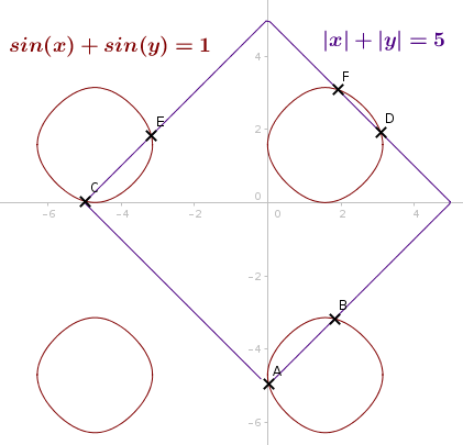
$\mathbf {B_{i+1} = {B_i} + \frac {\Delta f_i - s_i B_i \Delta x} {s_i \Delta x^T \Delta x} \Delta x^{T}}$

Figure 3: Intersection with absolute value function(Using Broyden Method)

Other Applications

Geometry

Root finding method can be used to find the tangents of a curve from a given point. For example - let the curve be $f(x, y) = 0$ , point $Q (x, y)$ is a point on the curve and we want to draw some tangent lines from point $P (x_k, y_k)$ . When we draw a line $PQ$ , slope of $PQ$ must be equal to the slope of curve at $Q$ . In mathematical terms we can write

$\frac {dy} {dx} = \frac {y - y_k} {x - x_k}$

The right hand side represents the slope of the line passing through two distinct points $P$ and $Q$ . The term in the left is derivative of curve which can be calculated as

$\frac {dy} {dx} = - \frac {\partial f(x, y) / \partial x} {\partial f(x, y) / \partial y}$

After some manipulation we will get another implicit curve equation as

$g(x, y) = \frac {dy} {dx} (x - x_k) - y + y_k = 0$

Now we can solve $f(x, y)$ and $g(x, y)$ to get some points $Qs$ on the curve where the slope of the curve is same as that of the line passing through $PQ$ .

Local minimum of function (Minimising cost function : Machine Learning)

This is a widely studied problem because we often need to find minimum or maximum value of a function in engineering, mathematics, statistics, machine learning and operation research. Here we only discuss minimization because maximizing $\mathbf {f(x)}$ is equivalent to minimizing $\mathbf {-f(x)}$ . In this problem we are interested in finding a stationary point $\mathbf{x^*}$ which statisfies $\mathbf {f(x^* + p) \ge f(x^*)}$ where $\mathbf {f(x^* + p)}$ is the value of function in the close neighborhood of $x^*$ . At the stationary point

$\mathbf { \frac {\partial f(x)} {\partial x_i} } = 0$

This partial derivatives will give us $n$ equations in $\mathbb{R^n}$ . We can solve these equations using the technique discussed above, or we can use some advanced optimization techniques such as BFGS, L-BFGS, or conjugate gradient.

Happy Reading!

Reference

[1] - Broyden, C. G. (October 1965), “A Class of Methods for Solving Nonlinear Simultaneous Equations”, Mathematics of Computation (American Mathematical Society) 19 (92): 577–593. doi:https://dx.doi.org/10.2307%2F2003941

[2] - Jorge Nocedal, Stephen J. Wright. “Numerical Optimization”